Bayesian Decision Task

The today's objective is to create a Bayesian classifier which will classify a single real measurement into one of two classes. We will assume the 'zero-one' loss function.

Problem formulation

The task is to design a classifier, which would distinguish between two letters K={'A', 'C'}, and that using only a single measurement:

x = (sum of pixel intensities in the left half of the image) - (sum of pixel intensities in the right half of the image)

This measurement (so-called feature) assigns a real number to each image. Let us assume that the percentage of letters 'A' and 'C' in a given dataset is known, i.e. we know the a priori probabilities p(A) and p(C). Further, let us assume that the conditional probabilities p(x|A) and p(x|C) are also known, that is the probabilities that a value x is measured if the letter is 'A' or 'C' respectively. Let probabilities p(x|A) and p(x|C) be Gaussian distributions with mean value and variance given for each class. Your task is to design a Bayesian classifier (strategy), i.e. a function k=q(x), which will minimize the risk (expected loss).

In this problem, the set of decisions D coincides with the set of hidden states K and the loss function W takes just two values: 0 for correctly recognized and 1 for incorrectly recognized letter. In this special case the classificator q expresses as (lecture notes Bayesian decision theory, slides 22-23)

q(x) = argmax_k p(k|x) = argmax_k p(k,x)/p(x) = argmax_k p(k,x) = argmax_k p(k) p(x|k),

where p(k|x) is called a posteriori probability of class k given the measurement x. Symbol argmax_k denotes finding k maximizing the argument.

Recall, that density of Gaussian (aka normal) probability of one variable is given by

where μ is mean value and σ is standard deviation (σ² is variance).

The task

Note: Recommended to go through tasks 1 and 4 before the exercise.

1. Show that in the case when p(x|A) and p(x|C) are Gaussian distributions the discriminative function of the Bayesian strategy is a quadratic function. Derive equations for coefficients of this quadratic discriminative function.
   
   Hint: For two-class classification problem, discriminative function is such that when it is positive the decision is in favor of first class and otherwise in favor of second class. Prove that for zero-one loss function, the optimal Bayesian strategy classifies x to class A if 
   
   p(x|A) / p(x|C) >= p(C) / p(A) 
   
   Substituting the equations for the Gaussian distribution for p(x|A) and p(x|C) and taking a logarithm of the whole equation, you will obtain a quadratic inequality with respect to x.
   
   
2. Download Matlab file data_33rpz_cv02.mat which contains images of letters 'A' and 'C', and parameters of the distributions p(A), p(C), p(x|A), p(x|C).
   
   Data description:

images	-	10x10x160, 160 images of size 10x10 pixels, depicting letters 'A' and 'C'
D1	-	a structure with parameters of the distribution p(x|A) = N(D1.Mean, D1.Sigma^2)
D1.Mean	-	mean value of p(x|A)
D1.Sigma	-	standard deviation of p(x|A)
D1.Prior	-	probability p(A), i.e. the percentage of 'A's in the dataset
D2	-	a structure with parameters of distribution p(x|C) = N(D2.Mean, D2.Sigma^2)
D2.Mean	-	mean value of p(x|C)
D2.Sigma	-	standard deviation of p(x|C)
D2.Prior	-	probability p(C), i.e. the percentage of 'C's in the dataset
labels	-	1x160, vector with ground-truth classification (to be used ONLY for evaluation of the classification error)
Alphabet	-	1x2, Alphabet = 'AC', the alphabet

2. For given values p(A), p(C) and parameters of p(x|A), p(x|C), compute the coefficients of the quadratic discriminative function (derived in task 1). Evaluate the discriminative function for each image, and classify it as either 'A' or 'C'. Display the classification results, e.g. show separately images classified as 'A' and as 'C'.
   
   
3. Compute the classification thresholds t₁ and t₂ such that the quadratic inequality a*x² + b*x +c >=0 for a<0 is expressed as two inequalities x≥t₁ and x≤t₂ and for a>0 is expressed as two inequalities x≤t₁ OR x≥t₂.
   
   
4. Write a function[risk,epsA,epsC,interA] = bayeserror(D1,D2), which returns the risk of the Bayesian strategy and the classification thresholds. The inputs are the structures D1 and D2 with the parameters of p(x|A), p(x|C), p(A) and p(C). Format of the structure is as in the task 2. The output shall be:

risk	-	risk/error of optimal Bayesian strategy
epsA	-	probability p(x|A) integrated over LC, where LC is the set where x is classified as 'C'.
epsC	-	probability p(x|C) integrated over LA, where LA is the set where x is classified as 'A'.
interA	-	one or two intervals defining the set LA

Hint: To integrate exponential functions you can use normcdf function from Statistics toolbox.

5. Having the correct classification of images (contained in the array labels), compute the actual classification errors for the given dataset. Compare the errors with the output of your bayeserror function.
   
   
6. Using the pgmm function from the stprtool toolbox display the probability densities and the classification thresholds t₁, t₂.

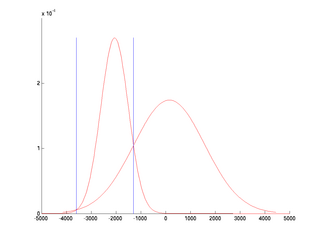
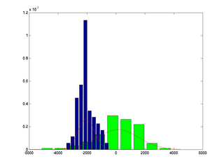
7. In a second figure, show empirical estimates of p(x|A) and p(x|B) computed from data. Use functions hist and bar. To obtain empirical estimates for distributions of continuous variable (they must integrate to 1) normalize the histograms as appropriate.
   Hint:
       [N, u] = hist(x);
       N = N / ( sum(N)*(u(2)-u(1)) ); % normalization (u – centers of bins)
   bar(u,N);
   or:
       [f, a] = ecdf(x);
   ecdfhist(f,a);
   
   

Contact the lab assistants if you have any questions.

Bonus task

This task is not compulsory. Work on bonus tasks deepens on your knowledge about the subject. Successful solution of a bonus task(s) will be positively reflected during the examination.

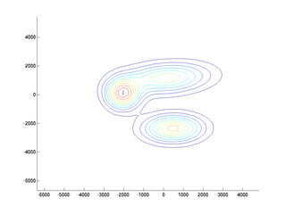
The data for this task can be downloaded from data_33rpz_cv02_bonus.mat. The task is analogous to the previous one, only there are now two measurements (features) and three classes. The second measurement is

y = (sum of pixel intensities in the upper half of the image) - (sum of pixel intensities in the lower half of the image)

The alphabet (i.e. the classes) now consists of three letters, 'A', 'C', and 'T'.

The task is to classify the input images into one of the three classes. Use both measurements x and y here. 
The density function p(x) = p(x|A)+p(x|C)+p(x|T) is visualized below (drawn using  pgmm function from the toolbox)

Output:

• Classification error of the optimal Bayesian strategy,
• Classification of input images, i.e. which image was assigned to which class – draw the images per class.

Hint:

Multivariate Gaussian distribution density is given by

• Use mnvpdf or pdfgauss function.

References

• Duda R., Hart P., Stock D.: Pattern Classification, 2001
• Michail I. Schlesinger, Vaclav Hlavac. Ten Lectures on Statistical and Structural Pattern Recognition. Kluwer Academic Publishers, 2002.   
• slides from lecture by Vaclav Hlavac and Jiri Matas.

---

Created by Martin Urban, last update 18.7.2011