Non-parametric estimation of probability distributions - Parzen windows

Last week, the problem was to estimate parameters of unknown probability distributions using the maximal likelihood method. We have assumed that the form of the distributions is known in advance (e.g. Gaussian), and we only had to estimate the parameters μ and σ. In many practical scenarios, however, the form of the distributions is unknown. In such cases, non-parametric estimation can be applied. Today, we will estimate the distributions with a method known as Parzen Windows.

(The term 'non-parametric estimation' might be misleading. In fact, the distribution parameters are again estimated by the maximal likelihood method, only the model of the distributions differs, and the maximum of likelihood is found numerically, not analytically)

Problem formulation

As in the last week's labs, the task is to create a Bayesian classifier for two classes of letters. Prior probabilities P(k) and probability distributions p(x|k) are unknown. A training set trn_2000 is provided, which allows you to estimate these unknown distributions. The distributions p(x|k) will be estimated using the Parzen window method. Once the distributions are known, a Bayesian classifier will be constructed and tested on an independent test set.

The letters will be classified using the following measurement:

x = (sum of pixel intensities in the left half of the image) - (sum of pixel intensities in the right half of the image)

The task

1. load the data file data_33rpz_cv05.mat into Matlab.
   
   The data file contains:

trn_2000	- images of the training set
tst	- images of the test set
Alphabet	- the alphabet

2. For each image from the training set, trn_2000, compute the measurement x. Store the measurements of different classes separately, i.e. make vectors X₁, X₂ for the two class problem.
3. Implement a function, y = my_parzen(x,X,sigma), which, using the method of Parzen windows, computes for a given x an estimation of probability p(x). X is a vector of training measurements for one of the classes. As the kernel function W(x) use normal distribution N(0, σ²).
   
   Hint: y = 1/n * Sum_i W(x-X(i)), where n is the length of vector X. Use normpdf() to calculate W.
   Note: In literature, the kernel functions can also be denoted as φ(x).
4. Use your my_parzen() function to estimate the probability distribution p(x|1). Show the normalized histogram of X₁ and the estimated p(x|1) in one figure. 
   
   • to compute the estimate of p(x|1) use your function: p(x|1) = my_parzen(x,X1,sigma)
   • iterate the variable x e.g. from min(X₁) to max(X₁), with a step of 100
   Show distribution estimates for three different choices of σ, e.g. sigma = [100,300,1000,2000].
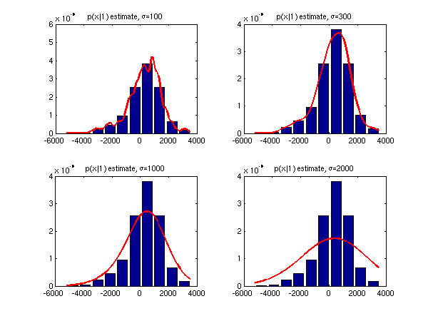
   Hint: the following code was used to draw the normalized histogram:
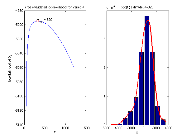
   [cdfF,cdfX] = ecdf(X); [cdfN,cdfC] = ecdfhist(cdfF,cdfX); bar(cdfC,cdfN);
5. Estimate the optimal value of σ using the maximal likelihood method
   The procedure:
1. Split the training set X₁ into two subsets X_1a and X_1b of identical cardinality
2. On the first subset, X_1a, estimate the distribution p(x|1). On the second (validation) subset, X_1b, compute the log likelihood L(σ), i.e.
   p(x|1) = my_parzen(x,X_1a,sigma)
   L(σ) = Sum_x log(p(x|1)), where the sum goes over all x from X_1b.
3. Repeat step 2 for different σ, e.g. sigma = 100, 200, ...., 1000.
4. Draw L(σ) as a function of σ, select the optimal value of σ.

Note: This procedure is in fact a simplified form of the so called crossvalidation method. If you like, you can implement the crossvalidation in its full form, e.g. splitting the training set into more than two subsets. To split the set you can use function crossval().


6. Follow steps 4-5 once again to estimate the distribution of p(x|2).
7. Use the estimated distributions p(x|1) and p(x|2) to create a Bayesian classifier. Estimate the a-priori  probabilities P(1) and P(2) on the training set, as you did last week. Compute the classification error on the test set tst.

Bonus task

• Follow steps 3-7 once again, only this time the kernel function W(x) will represent the uniform distribution:

W(x) = 1/h,	for abs(x) <=h/2,
W(x) = 0,	for abs(x) >h/2,

• where h denotes the width of the window. I.e. the parameter h corresponds to the parameter σ in normal distribution N(0,σ²).
• Once again follow steps 2-7, this time for two measurements

x = (sum of pixel intensities in the left half of the image) - (sum of pixel intensities in the right half of the image)
y = (sum of pixel intensities in the top half of the image) - (sum of pixel intensities in the bottom half of the image)

The kernel function will now be a 2D Gaussian distributions with diagonal covariance matrix cov = sigma^2*eye(2). Display the estimated distributions p(x|k).

References     

• Parzen window (Wikipedia)
• Parzen Windows (Duda,Hart)
• Metoda Parzenova okna (V. Hlaváč)
• Cross-validation (Wikipedia)

---

Created by Martin Urban and Karel Zimmerman, last updated 17.8.2011