The minimax task
In today's labs we will go through the so-called minimax decision strategy.
It solves a classification task where the apriori class probabilities are
unknown - hence we cannot derive the optimal Bayesian strategy.
The minimax problem
Let us consider the Bayesian classifier from
Lab 2 appllied to
the problem of recognition of car registration plates. Part of the registration
number reflects the administrative region, where the car is registered, e.g. the
letter 'A' stands for Prague. Would we know where our recognition system is
going to be located, we can estimate the class probabilities (e.g. count cars
passing at the given location over some time period) and use the Bayesian
strategy to obtain the optimal classifier. p('A'), the apriori class
probability of 'A' represents the relative number of passing cars that are
registered in Prague. For locations near Prague, p('A') will be higher than for
distant locations. But, in the case that we do not know where the system will
operate, the class probabilities are unknown. In such a case, the minimax
strategy gives us a classifier, which has optimal performance in the worst
situation (worst configuration of class probabilities).
As in the last labs, our single measurement x, on which the
classification will be based, is
x =
(sum of pixel intensities in the left half of the image) - (sum of pixel
intensities in the right half of the image)
The task
Let us simplify the task, and consider that only two letters occur on the
registration plates (i.e. we have two-class problem only). From the supplied
alphabet, choose whichever letters you would like. In the following, the two
letters will be denoted as 'A' and 'B'.
- Load the datafile data_33rpz_cv03_minmax.mat.
Its structure is identical to that of the last labs, except that the apriori
probabilities are unknown. Parameters of P(x|class) are stored in D
variable, the ordering of which corresponds to the Alphabet array.
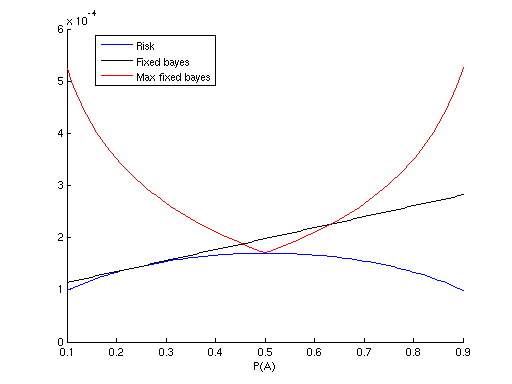
- Iterate over different values of apriori probability p('A') in <0,1>
inteval (e.g. {0.1, 0.2, ..., 0.9}), evaluate and show in a figure the
following:
- Risk of optimal Bayesian strategy, computed for each iterated p('A').
Hint: You can use the bayeserror() function you have
implemented before.
lab2_bayeserror, lab2_quadrdiscr
-
p(x|A) integrated over LB, where LB
is the range where x is classified into 'B', and p(x|B) integrated over LA, where LA
is the range where x is classified as 'A'.
Hint: these are also output arguments of your bayeserror() function.
- Risk of Bayesian strategy, which is optimal for pfixed('A')
= 0.25. What we would like to see here, is the risk of strategy optimal
for a choosen pfixed('A'), while the actual p('A') is
different (the iterated p('A')). In other words, what happens, when we
have assumed wrong apriori class probabilities. For example, when we would
like, wrongly, to solve the given problem as Bayesian, and state all the
(unknown) class probabilities as equal (by saying that all letters are
equaly probable).
Hint: Equation (3) from the first reference comes handy.
- For each iterated p('A') derive the optimal Bayesian strategy and
compute its worst-case risk, i.e. the risk if the actual p('A') differs
and is the worst possible. Display the maximal risk.
- Based on the results you have so far, find the minimax strategy and its
risk. The minimax strategy is the Bayesian strategy derived for p('A') with
lowest maximal risk (computed in 2.4).
Bonus task
This task is not compulsory.
Go through the chapter on non-Bayesian tasks in SH10 book (Schlesinger, Hlavac,
see reference below), especially the parts regarding solution of the minimax
task by linear programming (pages 25, 31, 35-38, 40-41, 46-47). Solve the problem
specified above using linear programming, as described on page 47.
Hints
- The domain of the measurement x is to be discrete. Therefore, first
discretise x into N equidistant bins.
- Represent the sought strategy (classification function) as a table α,
with α(i,k) corresponding to the probability of classification of bin
'i' to class 'k' (α (i,k) >= 0, sumk (α (i,k)) = 1).
- Reformulate the task in matrix form, according to equation 2.53 in SH10,
page 47
- Solve the task numerically, using linprog
function
- Show p(x|A) and p(x|B) of each bin in a single figure, show
also to which class are individual bins classified.
- Compare the results to the results of the task above.
References
- Minimax Task (short support text for labs)
- Michail I. Schlesinger, Vaclav Hlavac. Ten Lectures on Statistical and Structural Pattern Recognition.
Kluwer Academic Publishers, 2002.
Created
by Jan Šochman, last update 18.7.2011