Principal Component Analysis (PCA)

Principal component analysis (PCA) is a method for reduction of dimensionality of a feature space, i.e. we want to choose only few features (or measurements) from a large pool of measurements available. The problem is also called feature extraction. In today's labs, the PCA will be used to extract measurements from the 'space' of facial images.

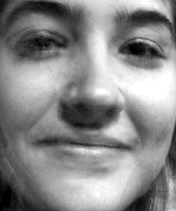
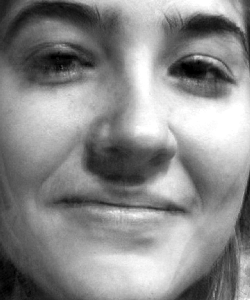
Let us have a set of facial images, with resolution of 300x250 pixels. Let's reorganise image pixels to a vector of length n = 75000 (= 300 * 250). This vector represents the image as a point in n dimensional space. I.e. we have n measurements on each image, each corresponding to a single pixel. Using PCA, we will find a representation of the images in a lower-dimensional space. The dimensionality of the new representation will be m, m << n. Facial images will then be classified in the m-dimensional space by nearest neighbour search.

Theory

Let us have k samples X_i ∈ Rⁿ (e.g. the vectorised images of faces). PCA searches for m < n vectors Y_j ∈ R^m , such that vectors X_i are approximated by linear combinations of Y_j with the lowest least squares residuum. I.e. each vector X_i is approximated by a linear combination of Y_js. Let us denote the approximation by Z_i.

Z_i = ∑_j w_ij Y_j, i = 1, ... , k; j = 1, ... , m
the residuum

g(Y_j, w_ij) = ∑_i || X_i - Z_i ||²

is minimised. Each input vector X_i is represented by only by m coefficents w_ij, j = 1, ... ,m of the linear combination, i.e. by an m-dimensional vector.
The vectors Y_j are found as eigenvectors of matrix S = XX^T. First m eigenvectors, corresponding to m highest eigenvalues are used. The matrix X is of dimension n×k and stores the input measurements: i-th column of X contains X_i.
The coefficients w_ij of the linear combination are then found as dot products w_ij = X_i^T Y_j

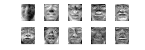
In the case of representation of images of faces, the eigenvectors Y_j are dubbed eigenfaces.

A useful trick

As is often the case when working with images, the matrix S soon becomes too large to be represent in a computer's memory. In our case, S would need about 45 GB. Therefore, we emplooy the following trick [1, 3].

In the original task formulation, eigenvectors of S = XX^T (n×n) are computed (n = 75000).

Su = λu

Instead of S, let us construct a smaller matrix T = X^TX (k×k). The relation between eigenvectors of S and T is

Tv = (X^TX)v = λv
X(X^TX)v = Xλv = λ(Xv)
S(Xv) = λ(Xv)

Therefore, if we look for first m ≤ k eigenvectors of S only, it is sufficient to compute eigenvectors of much smaller matrix T. Multiplying them by matrix X we obtain the desired eigenvectors of S.

Summary

Here we list the operations which you will need to implement. We will denote the original n-dimensional input space as image-space, and the reduced m-dimensional space as the face-space.

Transformation from image-space to face-space - Dot-product of an input image X_i with each of the eigenvectors Y_j, j = 1, ... ,m

Transformation from face-space to the image-space - the linear combination: weigted sum of eigenvectors, the weights were given by the previous operation.

Partial image reconstruction - the transformation from face-space to image-space, but using only several first eigenvectors.

Learning of a face - transformation of input image to face-space and storing the m-dimensional vector of weights.

Recognition of a face - transformation of input image to face-space, and finding the nearest neighbour of the m-dimensional representaiton. If the closest face representation is closer than a threshold, return the found identity, otherwise return 'unknown' face.

How is an image face-like? - Transform the image to face-space and back. Compute the mean squared error between the input and the reconstructed images. If the error is large, the image does not resemble a face.

The task

Download images of faces (data_33rpz_cv12.mat). The file contains training (structure trn_data) and test (structure tst_data) data. The structures contain fields images (with images) and names (with names of persons on the images, i.e. identifiers for the recognition problem).
Implements PCA using the above described trick.. Use images from trn_data as input, to find the eigenvectors.
Tip 1: Eigenvectors and eigenvalues are in Matlab computed by function eig.
Tip 2: Normalise the computed eigenvectors to unit length.
Display the eigenvectors (eigenfaces) as images. I.e. reorganise vectors Y to matrices of the same size as the input images.

...
What does the first eigenvector correspond to?
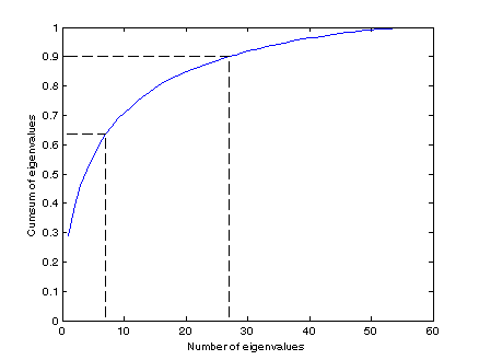
Plot the cumulative sum of normalised (i.e. that they sum to one) eigenvalues (skip the first one).
Depending on the task, the number of eigenvectors used to approximate the data is chosen so that the cumulative sum of their respective eigenvalues is about 65%-90% of the sum of all eigenvalues.

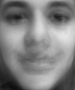
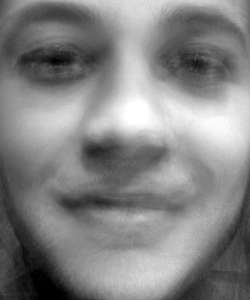
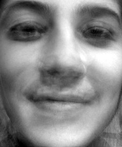
Draw partial reconstructions of a selected face, while increasing the number of used eigenvectors
Using the nearest neighbour classification in the face-space, classify the images from tst_data. Experiment with the number of eigenvectors (the dimensionality m of the face-space) Print the classification error.

Bonus task

What to do next? With the knowledge gained in this term, you can

... experiment with another (better ?) classifier in the face-space,
... try to align the faces first, i.e. before computing the PCA. (Use another data file, where the faces are not so tightly clipped, so you have some space to crop the images. For inspiration, see [2]),
... experiment with PCA on letters, which were used on previous labs (e.g. with data for Adaboost labs),
... compare PCA with Independent Component Analysis (ICA),
... implement a simple (although slow) face detector (see end of Summary Section),
...

Any of the given topics is considered a bonus task. The formulations are vague intentionally, the precise task formulation, and specification of inputs, is part of the task.

References

[1] Eigenfaces for recognition talk

[2] Face alignment for increased PCA precision

[3] Turk, M. and Pentland, A. (1991). Eigenfaces for recognition. The Journal of Cognitive Neuroscience, 3(1): 71-86.

Created by Jan Šochman. Last updated 18.7.2011