Contents

fig = 0;

Show spectrum of common 2D signals

%TODO {
% - Implement a 2D signal generator. It will generate common 2D signals
%   (constant, harmonic, square, circ, Gaussian, Gabor). Use template
%   [image_generator.m].
%
% - Implement a function, which "nicely" visualizes the magnitude frequency
%   spectrum (hint: use logarthmic scaling). Use template
%   [show_spectrum.m].
%
% Feel free to change the parameters of the 2d-signals below, e.g.
% frequencies, spatial extent, etc. Experiment with displaying spectrum in
% pseudo-colors using a different colormap, e.g. 'jet'.
%
% }

%constant signal
x = image_generator('constant',[128,128],1);
X = fft2(x);

fig=fig+1; figure(fig); imagesc(x); colormap gray; axis image; title('Constant signal')
fig=fig+1; figure(fig); show_spectrum(X,'gray'); title('Constant signal magnitude spectrum')

%harmonic signal (horizontal frequency only)
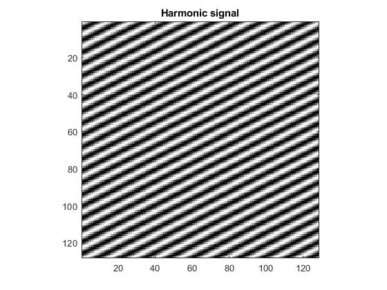
x = image_generator('harmonic',[128,128], 20*pi/128, 0*pi/128, 0);
X = fft2(x);

fig=fig+1; figure(fig); imagesc(x); colormap gray; axis image; title('Harmonic signal')
fig=fig+1; figure(fig); show_spectrum(X,'gray'); title('Harmonic signal magnitude spectrum')

%harmonic signal (horizontal and vertical frequency only)
x = image_generator('harmonic',[128,128], 20*pi/128, 40*pi/128, 0);
X = fft2(x);

fig=fig+1; figure(fig); imagesc(x); colormap gray; axis image; title('Harmonic signal')
fig=fig+1; figure(fig); show_spectrum(X,'gray'); title('Harmonic signal magnitude spectrum')

%harmonic signal (Nyquist frequency)
x = image_generator('harmonic',[128,128], pi, pi, 0);
X = fft2(x);

fig=fig+1; figure(fig); imagesc(x); colormap gray; axis image; title('Harmonic signal at Nyquist frequency')
fig=fig+1; figure(fig); show_spectrum(X,'gray'); title('Harmonic signal magnitude spectrum')

%square
x = image_generator('square',[512,512],10);
X = fft2(x);

fig=fig+1; figure(fig); imagesc(x); colormap gray; axis image; title('Square')
fig=fig+1; figure(fig); show_spectrum(X,'gray'); title('Square magnitude spectrum')

%circ
x = image_generator('circ',[512,512],15);
X = fft2(x);

fig=fig+1; figure(fig); imagesc(x); colormap gray; axis image; title('Circ')
fig=fig+1; figure(fig); show_spectrum(X,'gray'); title('Circ magnitude spectrum')

%Gaussian
x = image_generator('Gaussian',[512,512],5);
X = fft2(x);

fig=fig+1; figure(fig); imagesc(x); colormap gray; axis image; title('Gaussian')
fig=fig+1; figure(fig); show_spectrum(X,'gray'); title('Gaussian magnitude spectrum')

%Gaussian with a wider support
x = image_generator('Gaussian',[512,512],50);
X = fft2(x);

fig=fig+1; figure(fig); imagesc(x); colormap gray; axis image; title('Gaussian')
fig=fig+1; figure(fig); show_spectrum(X,'gray'); title('Gaussian magnitude spectrum')

%Gabor filter
x = image_generator('Gabor',[512,512],0.15*pi, 0.1*pi, 50);
X = fft2(x);

fig=fig+1; figure(fig); imagesc(x); colormap gray; axis image; title('Gabor')
fig=fig+1; figure(fig); show_spectrum(X,'gray'); title('Gabor magnitude spectrum')

Spectrum of a photo, importance of a phase spectrum

x0 = imread('Lenna.png');
x0 = double(sum(x0,3)/3);

X0 = fft2(x0);

%TODO {
%  - Switch phase of the specrum to constant 0. X1 will be the spectrum of
%    the image having the same magnitude as the spectrum of the input image,
%    but a constant (zero) phase.
%
%  X1 =
%}
x1 = ifft2(X1); %inverse fft (result is an image)

%TODO {
%  - Switch magnitude of the specrum to constant 1. X2 will be the spectrum
%    of the image having the same phase as the spectrum of the input
%    image, but a constant magnitude (a_i = 1 for all frequencies).
%
%  X2 =
%}
x2 = real(ifft2(X2)); %inverse fft (result is an image)

fig = fig+1;
figure(fig);
image(x0); colormap gray;
axis image; title('Input image');

fig = fig+1;
figure(fig);
show_spectrum(X0,'gray');
axis image; title('Magnitude spectrum');

fig = fig+1;
figure(fig);
imagesc(x1); set(gca,'clim',[0,255]); colormap gray
axis image; title('Reconstructed image - Altered spectrum phase');

fig = fig+1;
figure(fig);
imagesc(x2); colormap gray
axis image; title('Reconstraucted image - Altered spectrum magnitude');

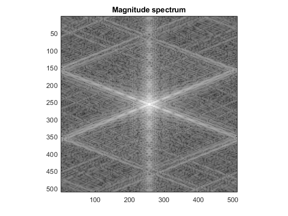
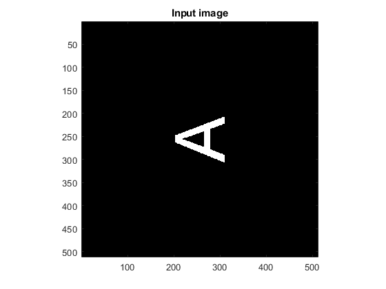
Spectrum of translated/rotated image

x = imread('A_black.png');

fig = fig+1; figure(fig);
imagesc(x); colormap gray; title('Input image');
axis image;

X = fft2(x);

fig = fig+1; figure(fig);
show_spectrum(X,'gray'); title('Magnitude spectrum');
axis image;

%TODO {
% Translate the image by 100px horizontally and by 50 px vertically, show
% the image and the magnitude spectrum
%
%}

%TODO {
% Rotate the image by 90 degrees counterclockwise, show the image and the
% magnitude spectrum
%
%}

%TODO {
% Rotate the image by 45 degrees clockwise, show the image and the
% magnitude spectrum  - Use rotated image "A_black_45.png"
%
%}

Low/high pass filtering in frequency domain (OPTIONAL)

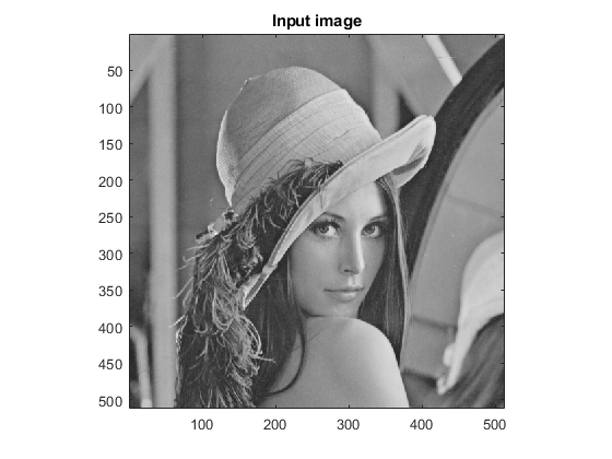
x = imread('Lenna.png');
x = double(sum(x,3)/3);

fig = fig+1; figure(fig);
image(x); colormap gray;
axis image; title('Input image');

X = fft2(x);

fig = fig+1; figure(fig);
show_spectrum(X,'gray'); cl = get(gca, 'clim');
axis image; title('Magnitude spectrum');

%TODO {
% Construct a blurred image by attenuating magnitudes of high frequencies.
% - Construct a Gaussian filter G of the same size as the image and centered
%   at image center (use sigma=20)
% - Multiply the spectrum with the Gaussian filter G
%
% Construct a high-pass filtered image by removing removing low frequencies
% - Construct a circular filter which cuts off all frequencies below pi/8
% - Multiply the spectrum with the circular filter H
%
% %low pass
% G = ...
% Yg = ... %low-pass filtered spectrum
%
%
% %high pass
% H = ...
% Yh = ... %high-pass filtered spectrum
%
%}

%low pass
fig = fig+1; figure(fig);
imagesc(G); colormap('gray')
axis image; title('Gaussian Filter in frequency domain')

fig = fig+1; figure(fig);
show_spectrum(Yg,'gray',cl);
axis image; title('Filtered magnitude spectrum (Low-pass)');

yg = real(ifft2(Yg));

fig = fig+1; figure(fig);
image(yg); colormap gray
axis image; title('Low-pass filtered image');

% high pass
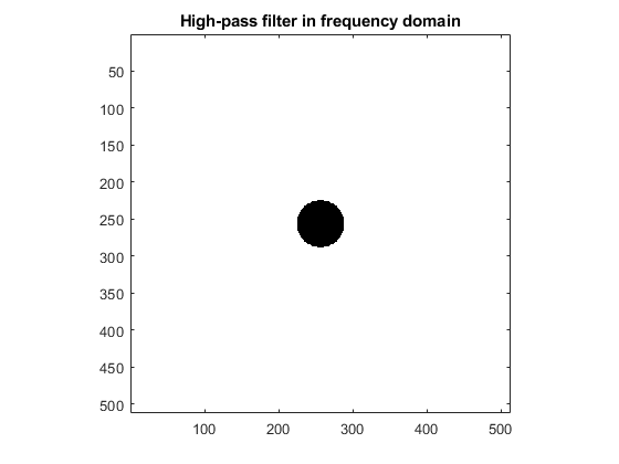
fig = fig+1; figure(fig);
imagesc(H); colormap gray
axis image; title('High-pass filter in frequency domain')

fig = fig+1;figure(fig);
show_spectrum(Yh,'gray',cl);
axis image; title('Filtered magnitude spectrum (High-pass)');

yh = real(ifft2(Yh));

fig = fig+1; figure(fig);
image(yh); colormap gray
axis image; title('High-pass filtered image');

Published with MATLAB® R2019b