We will assume the normal distribution of the class probability density functions: p(x|k) ~ N(μk, σk). To estimate the densities, only their parameters, μk and σk, have to be estimated. We will find their maximum likelihood estimates.
Estimated apriori probabilities and probability density functions will be used to build a Bayesian classifier which, in turn, will be applied to the test set.
The task
- Load the datafile data_33rpz_cv04.mat
into Matlab.
- For all the training sets do following:
- Compute the apriori probabilities P(A) a P(C).
- Compute the maximum likelihood estimates of the
parameters μk
and σk
of the distributions p(x|A)
and p(x|C).
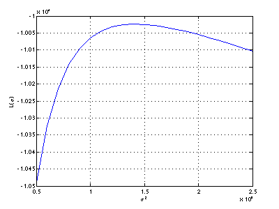
The estimation is explained in [2]. - For μk computed in 2.2 plot the log-likelihood function L
from equation (2) in support text [2] (or [1], eq 5, page 87) as a function of
σk. It
is enough to do it for one class only, e.g. class A.
- Plot the estimates of p(x|A) and p(x|C) into one
graph together with normalised histogram of the training set.
- Use the estimates to build a Bayesian classifier. Apply the
classifier to the test set and compute the classification error.
Hint: use the implementation from previous labs.
Bonus task
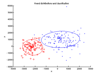
- Repeat steps 2.1, 2.2 and
4 for two-dimensional measurements X = (x, y)T.
- As in step 3, display the distribution estimates (use the
function pgauss)
and the test set (function ppatterns).
Recommended literature
[1] Richard O. Duda, Peter E. Hart, David G. Stork. Pattern Classification.[2] Maximum Likelihood Parameter Estimation (short support text for labs)
[3] Maximálně věrohodný odhad (longer text in Czech, includes multi-dimensional normal distribution estimates (13,14) needed for bonus task)
Created by Jan Šochman. Last modification 18.7.2011