The Perceptron Algorithm

The task today is to implement the perceptron algorithm for learning of a linear classifier. Once implemented, the algorithm will also be used for learning of a non-linear extension of the classifier, for the case of a quadratic discriminant function.

Task formulation

The task:

1. Implement the perceptron algorithm. Test its functionality on synthetic two-dimensional linearly separable data. For data creation use the createdata script.
   Output:
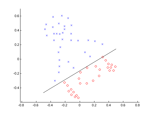
   • Show the decision boundary of the linear classifier you have found (a line), and the classified data. Use functions pline and ppatterns.
   • Plot evolution of the classification error as the learning proceeds. The error should generally decrease, but it does not have to be monotonous.
   Question: What can you tell about the solution? Is it optimal? In what sense?
   
   
2. Test the algorithm for data, which cannot be linearly separated (e.g. the XOR problem).
   Question: What's happening in the non-separable case?
   
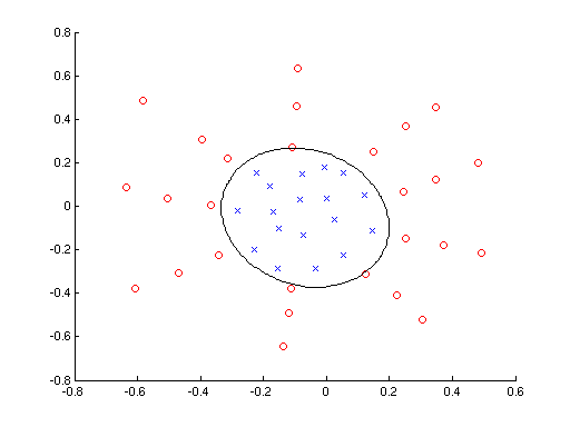
3. Extend the perceptron algorithm for the case of quadratic discriminant function. Demonstrate the functionality on a simple example.
   Hint:  For visualisation use pboundary function. This function takes a single parameter (model), which is expected to be a struct. It's member .fun refers to your classification function (e.g.. 'classif_quadrat_perc'), which is defined as

The function is called automatically by the visualisation function, and it's role is to classify the supplied test_data  (in our case 2D data) to two classes (i.e. the classif output is either 1 or 2). Parameters of the classifiers should be stored in the model parameter, which is the same one as the one passed to the pboundary function. In our case, the model will contain parameters of the current state of the quadratic classifier.

Bonus task:

The algorithm: Vector α₁ is any vector from convex hull of set {x^j, j ∈ J}, e.g. one of the vectors x^j, j ∈ J. If vector α_t has already been computed, α_t+1 is obtained using the following rules:

1. A misclassified vector x^j, j ∈ J is sought, which satisfies 
   <α,x^j> ≤ 0
   
2. If such x^j does not exist, the solution to the task has been found, and α_t+1 equals to α_t.
3. If such x^j does exist, it will be denoted as x_t. Vector α_t+1 then lies on a line passing through α_t and x_t . From all the points on the line, α_t+1 is the closest one to the origin of the coordinate system. In other words
   
   α_t+1 = (1 - k) α_t + k x_t
   where
   k = argmin_k | (1 - k) α_t + k x_t |.

References: