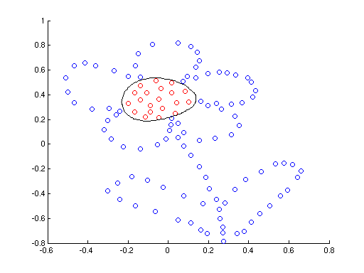
Hint: For visualisation of the decision boundary use function pboundary in the same way as it was used for the Perceptron. Implement the SVM classification function, i.e. replace your classif_quadrat_perc with classif_rbf_svm, wich will have the same arguments.
Input to the function classif_rbf_svm are test data, supplied automatically by the pboundary function, and a struct model, which contain whichever data you need for specification of the classifier. The function outputs a vector of the same length as the test data, which contains +1 or -1 depending on which class were the test data classified to.
x = (sum of pixel
intensities in the left
half of the image) - (sum of pixel intensities in the right half of the
image)
y = (sum of pixel intensities in the top half of the image) - (sum of pixel intensities in the bottom half of the image)
- Experiment with different parameters C and σ.
[2] Lecture slides
[3] Quadratic programming
[4] Christopher J. C. Burges. A Tutorial On Support Vector Machines for Pattern Recognition.
Created by Jan Šochman, last update 18.7.2011
y = (sum of pixel intensities in the top half of the image) - (sum of pixel intensities in the bottom half of the image)
Bonus task
In the character classification task find the optimal value of parameter σ of the RBF kernel using the cross-validation (see labs Parzen windows).
References
[1] Text of exercise from previous course.[2] Lecture slides
[3] Quadratic programming
[4] Christopher J. C. Burges. A Tutorial On Support Vector Machines for Pattern Recognition.
Created by Jan Šochman, last update 18.7.2011