Support Vector Machines classifier

Introduction

Let ${\cal T}_{XY} = \{(x_1,y_1),\ldots,(x_l,y_l)\}$ be a training set of observable vectors $x_i\in{\cal X}\subseteq{\mathbb{R}}^n$ and corresponding binary hidden states $y_i\in\{1,2\}$. The binary classifier $q\colon {\cal X}\rightarrow \{1,2\}$ assigns the vector $x\in{\cal X}$ to a hidden state $y\in\{1,2\}$ such that

$$q(x) = \left \{ \begin{array}{rcl} 1 & \mbox{for} & f(x)... ...:,\\ 2 & \mbox{for} & f(x)< 0\:,\\ \end{array} \right .$$

The $f\colon{\cal X}\rightarrow {\mathbb{R}}$ is the discriminant function which has to be trained from the training set ${\cal T}_{XY}$. In the case of the SVM classifier the discriminant function has the following form

$$f(x) = \sum_{i\in{\cal I}_{SV}}\alpha_i k(x,x_i) + b \:,$$

where ${\cal I}_{SV}\subseteq\{1,\ldots,l\}$ are indices of a subset of training vectors, $k\colon{\cal X}\times{\cal X}\rightarrow {\mathbb{R}}$ is a kernel function, $\alpha = [\alpha_1,\ldots,\alpha_m]^T\in{\mathbb{R}}^m$ is a weight vector and $b\in{\mathbb{R}}$ is a bias.

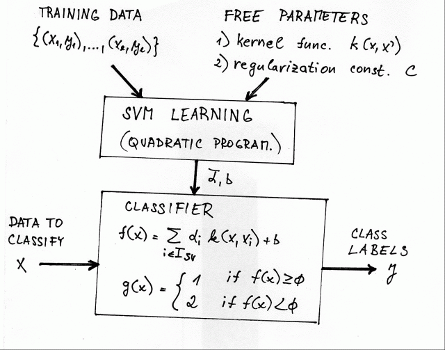
The training stage of the SVM classifier is transformed to a quadratic programming optimization task. The input of the optimization task is the training set ${\cal T}_{XY}$, kernel function $k$ and a regularization constant $C\in{\mathbb{R}}^+$. The output of the optimization is the weight vector $\alpha$ and the bias $b$. Thus the SVM training takes care of determination of the parameters $\alpha$, $b$. The remaining free parameters, i.e. kernel function $k$ and the regularization constant $C$, must be selected based on another principle. A common practice is to minimize the cross-validation estimate of the classification error with respect to these free parameters.

Figure 1: Support Vector Machines learning.

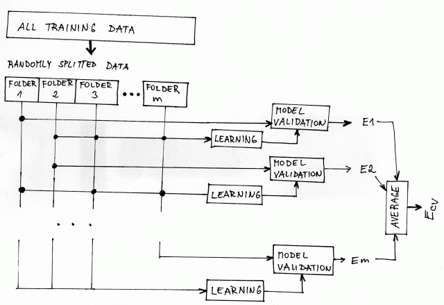
The cross-validation estimate of the classification error is computed as follows. The training set ${\cal T}_{XY}=\{(x_1,y_1),\ldots,(x_l,y_l)\}$ is randomly and uniformly partitioned into $m$ subsets ${\cal T}_{XY}^i$, $i=1,\ldots,m$ such that ${\cal T}_{XY} = {\cal T}_{XY}^1\cup \ldots \cup{\cal T}_{XY}^m$. The computation of the cross-validation error involves:

• Repeat for $i=1,\ldots, m$:
  1. Make the testing set ${\cal T}_{XY}^{tst}$ and the training set ${\cal T}_{XY}^{trn}$ as
     
     $${\cal T}_{XY}^{tst} = {\cal T}_{XY}^i\qquad \mbox{and}\qqu... ...T}_{XY}^{trn} = {\cal T}_{XY} \setminus {\cal T}_{XY}^i\:.$$
     
     

  2. Train the classifier $q$ on the training set ${\cal T}_{XY}^{trn}$.
  3. Compute classification error $\varepsilon _i$ on the testing set ${\cal T}_{XY}^{tst}$.
• Compute the cross-validation error
  
  $$\varepsilon _{CV} = \frac{1}{m} \sum_{i=1}^m \varepsilon _i\:.$$
  
  

The number $m$ is a trade of between the precision of the cross-validation estimate and the time requirements on the computation. The limit case $m=l$ is called the leave-one-out method.

Figure 2: Cross-validation.

Task assignment

1. Implement the cross-validation procedure for tuning of the SVM parameters (kernel function and the regularization constant). Use the Radial Basis Function (RBF) kernel $k(x,x')=\exp(-\frac{\Vert x-x'\Vert^2}{2\sigma^2})$ with parameter $\sigma$.
2. Apply the cross-validation procedure to train a binary SVM classifier for Brodatz textures $1$ and $2$ [brodatz1_trn.mat]. Plot the cross-validation estimate of the classification error with respect to the tuned parameters.
3. Validate the resulting SVM classifier on the testing data [brodatz1_tst.mat].

Useful functions

svm_exp1	Example on training SVM and using SVM classifier.
crossval	Partitions data for cross-validation.
svmlight or smo	Training procedures for binary SVM classifiers.