A better approach should take the information of more pixels into account. This could be achieved by comparing local neighborhoods of corners through intensity cross-correlation. As a neighborhood a small window of
![]() pixels centered around the corner could be taken. For the points
pixels centered around the corner could be taken. For the points ![]() and
and ![]() the similarity measure is obtained as follows:
the similarity measure is obtained as follows:
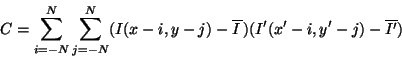 |
(D3) |
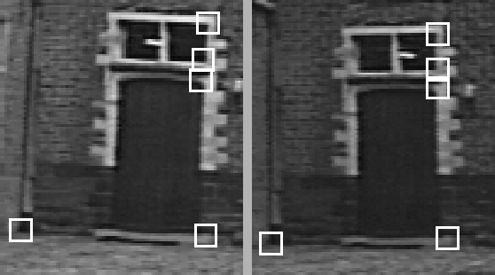
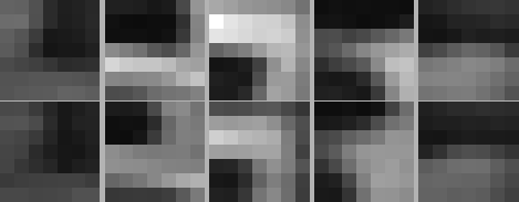
In figure 4.2 corresponding parts of two images are shown. In each the position of 5 corners is indicated. In figure 4.3 the neighborhood of each of these corners is shown. The intensity cross-correlation was computed for every possible combination. This is shown in Table 4.1. It can be seen that in this case the correct pair matches all yield the highest cross-correlation values (i.e. highest values on diagonal). However, the combination 2-5, for example, comes very close to 2-2. In practice, one can certainly not rely on the fact that all matches will be correct and automatic matching procedures should therefore be able to deal with important fraction of outliers. Therefore, further on robust matching procedures will be introduced.
If one can assume that the motion between two images is small (which is needed anyway for the intensity cross-correlation measure to yield good results), the location of the feature can not change widely between two consecutive views. This can therefore be used to reduce the combinatorial complexity of the matching. Only features with similar coordinates in both images will be compared. For a corner located at ![]() , only the corners of the other image with coordinates located in the interval
, only the corners of the other image with coordinates located in the interval
![]() .
. ![]() and
and ![]() are typically
are typically ![]() or
or ![]() of the image.
of the image.