Refining structure

The structure is refined using an Iterated Extended Kalman Filter for each point. The notation $q_k$ is used to indicate a quantity $q$ in view $k$, and $\hat{q}_k$ to indicate a estimation based on the observations up to view $k$. The observation equation is:

$$\left[ \begin{array}{c} x_k \\ y_k \end{array} \right] = {\t... ...tt M} \\ {\tt P}_{k2} {\tt M} \end{array} \right] + {\tt w}_k$$ (E4)

where $x_k$ and $y_k$ are the image coordinates of the observed feature, ${\tt M}$ is the observed 3D point and ${\tt w}_k$ is zero-mean Gaussian noise (uncorrelated over the images). ${\tt P}_{ki}$ is the $i$th row of the projection matrix ${\bf P}_k$. The update equations for state vector and covariance matrix are

$${\tt\hat{M}}_k = {\tt\hat{M}}_{k-1} + {\bf W} \nu_k$$ (E5)

$${\tt\Lambda}_k = {\tt\Lambda}_{k-1} - {\bf W} {\bf S}_k {\bf W}^\top$$ (E6)

where the Kalman gain matrix, innovation vector, and innovation covariance are

$${\bf W} = \nu_{k-1} \nabla {\tt p}_{\tt M}^\top {\bf S}_k^{-1}$$ (E7)

$$\nu_k = \left[ \begin{array}{c} x_k \\ y_k \end{array} \right] - {\tt p}\left( {\tt\hat{M}}_{k-1} \right)$$ (E8)

$${\bf S}_k = \nabla {\tt p}_{\tt M} {\tt\Lambda}_{k-1} \nabla {\tt p}_{\tt M}^\top + {\bf R}_k$$ (E9)

respectively, and ${\bf R}$ is the covariance matrix for the observed image points ${\tt m}$. The Jacobian $\nabla {\tt p}_{\tt M}$ of the non-linear observation equation 5.4 is evaluated at ${\tt\hat{M}}_{k-1}$

$$\nabla {\tt p}_{\tt M} = \left[ \begin{array}{ccc} \frac{\p... ...rtial Y} & \frac{\partial p_y}{\partial Z} \end{array}\right]$$ (E10)

whose $ij$-th element is

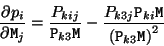$$\frac{\partial p_i}{\partial {\tt M}_j} = \frac{P_{kij}}{{\t... ... \frac{P_{k3j}{\tt P}_{ki} {\tt M}}{{({\tt P}_{k3}{\tt M})}^2}$$ (E11)

Within an IEKF, the update cycle in equations 5.5 and 5.6 is repeated for a number of iterations with $\nabla {\tt p}_{\tt M}$ evaluated at the current value of ${\tt\hat{M}}_k$ on each iteration. Beardsley et al [9] proposed 3 iterations.

If a 3D point is not observed the position is not updated. In this case one can check if the point was seen in a sufficient number of views to be kept in the final reconstruction. This minimum number of views can for example be put to three. This avoids to have an important number of outliers due to spurious matches.