


Next: Deviations from the camera
Up: The projection matrix
Previous: The projection matrix
Contents
The homographies that will be discussed here are collineations from
 . A homography
  describes the transformation from one plane to another. A number of special cases are of interest, since the image is also a plane. The projection of points of a plane into an image
  can be described through a homography
 . The matrix representation of this homography is dependent on the choice of the projective basis in the plane.
As an image is obtained by perspective projection, the relation between points
 belonging to a plane
  in 3D space and their projections
 in the image is mathematically expressed by a homography
. The matrix of this homography is found as follows. If the plane is given by
in the image is mathematically expressed by a homography
. The matrix of this homography is found as follows. If the plane is given by
![${\tt\Pi} \sim [{\tt\pi}^\top \, 1]^\top$](img336.gif) and the point
of is represented as
and the point
of is represented as
![${\tt M}_{\tt\Pi} \sim [{\tt m}^\top_{\tt\Pi} \, 1]^\top$](img337.gif) , then
belongs to if and only if
, then
belongs to if and only if
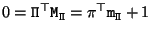 . Hence,
![\begin{displaymath}
{\tt M}_{\tt\Pi} \sim \left[ \begin{array}{c} {\tt m}_{\tt\P...
...{\tt\pi}^\top \end{array} \right] {\tt m}_{\tt\Pi}
\enspace .
\end{displaymath}](img339.gif) |
(C13) |
Now, if the camera projection matrix is
![${\bf P}_i=[{\bf A}_i \vert {\tt a}_i ]$](img340.gif) , then the projection
of
onto the image is
, then the projection
of
onto the image is
Consequently,
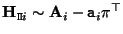 .
.
Note that for the specific plane
![${\tt\Pi}_{\tt REF}= [0\,0\,0\,1]^\top$](img346.gif) the homographies are simply given by
the homographies are simply given by
 .
.
It is also possible to define homographies which describe the transfer from one image to the other for points and other geometric entities located on a specific plane. The notation
 will be used to describe such a homography from view to
  for a plane . These homographies can be obtained through the following relation
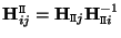 and are independent to reparameterizations of the plane (and thus also to a change of basis in
  ).
).
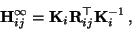
In the metric and Euclidean case,
 and the plane at infinity is
![${\tt\Pi}_\infty=[0 0 0 1]^\top$](img351.gif) . In this case, the homographies for the plane at infinity can thus be written as:
. In this case, the homographies for the plane at infinity can thus be written as:
 |
(C15) |
where
 is the rotation matrix that describes the relative orientation from the
  camera with respect top the
  one.
one.
In the projective and affine case, one can assume that
![${\bf P}_1 = [{\bf I}_{3 \times 3} \vert {\tt0}_3]$](img356.gif) (since in this case
(since in this case  is unknown). In that case, the homographies
 for all planes; and thus,
 . Therefore
  can be factorized as
![\begin{displaymath}
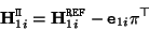
{\bf P}_i = [ {\bf H}_{1i}^{\tt REF} \vert {\tt e}_{1i} ]
\end{displaymath}](img361.gif) |
(C16) |
where  is the projection of the center of projection of the first camera (in this case,
![$[0 \, 0\, 0\, 1]^\top$](img256.gif) ) in image . This point is called the epipole, for reasons which will become clear in Section 3.3.1.
) in image . This point is called the epipole, for reasons which will become clear in Section 3.3.1.
Note that this equation can be used to obtain
 and from , but that due to the unknown relative scale factors can, in general, not be obtained from
and . Observe also that, in the affine case (where
), this yields
and from , but that due to the unknown relative scale factors can, in general, not be obtained from
and . Observe also that, in the affine case (where
), this yields
![${\bf P}_i = [ {\bf H}_{1i}^\infty \vert {\tt e}_{1i} ]$](img363.gif) .
.
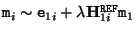
Combining equations (3.14) and (3.16), one obtains
 |
(C17) |
This equation gives an important relationship between the homographies for all possible planes. Homographies can only differ by a term
![${\tt e}_{1i} [{\tt l-\pi}']^\top$](img365.gif) .
This means that in the projective case the homographies for the plane at infinity are known up to 3 common parameters (i.e. the coefficients of
.
This means that in the projective case the homographies for the plane at infinity are known up to 3 common parameters (i.e. the coefficients of
 in the projective space).
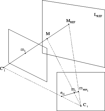
Equation (3.16) also leads to an interesting interpretation of the camera projection matrix:
In other words, a point can thus be parameterized as being on the line through the optical center of the first camera (i.e.
![$[0 0 0 1]^\top$](img371.gif) ) and a point in the reference plane
) and a point in the reference plane
 . This interpretation is illustrated in Figure 3.4.
Figure 3.4:
A point  can be parameterized as
 . Its projection in another image can then be obtained by transferring
  according to
 (i.e. with
 ) to image and applying the same linear combination with the projection
  of
of  (i.e.
(i.e.
 ).
).
 |
Next: Deviations from the camera
Up: The projection matrix
Previous: The projection matrix
Contents
Marc Pollefeys
2000-07-12
![$\displaystyle [ {\bf I}_{3 \times 3} \vert {\tt0}_3] \left[\begin{array}{c} {\tt m} \\ 1 \end{array}\right] = {\tt m}$](img367.gif)
![$\displaystyle [ {\bf H}_{1i}^{\tt REF} \vert {\tt e}_{1i} ]
\left[\begin{array}...
...\tt m} \\ 1 \end{array}\right] = {\bf H}_{1i}^{\tt REF} {\tt m} + {\tt e}_{1i}$](img369.gif)
![$\displaystyle \lambda {\bf H}_{1i}^{\tt REF} {\tt m}_1 + {\tt e}_{1i} = {\bf P}...
...\end{array}\right] + \left[\begin{array}{c} {\tt0}_3 \\ 1 \end{array}\right] )$](img370.gif)
![$\displaystyle [{\bf A}_i \vert {\tt a}_i ]
\left[ \begin{array}{c} {\bf I}_{3 \times 3} \\ -{\tt\pi}^\top \end{array} \right] {\tt m}_{\tt\Pi}$](img343.gif)