Two view geometry

In this section the following question will be addressed: Given an image point in one image, does this restrict the position of the corresponding image point in another image? It turns out that it does and that this relationship can be obtained from the calibration or even from a set of prior point correspondences.

Although the exact position of the scene point ${\tt M}$ is not known, it is bound to be on the line of sight of the corresponding image point ${\tt m}$. This line can be projected in another image and the corresponding point ${\tt m}'$ is bound to be on this projected line ${\tt l}'$. This is illustrated in Figure 3.5.

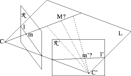
Figure 3.5: Correspondence between two views. Even when the exact position of the 3D point ${\tt M}$ corresponding to the image point ${\tt m}$ is not known, it has to be on the line through ${\tt C}$ which intersects the image plane in ${\tt m}$. Since this line projects to the line ${\tt l}'$ in the other image, the corresponding point ${\tt m}'$ should be located on this line. More generally, all the points located on the plane defined by ${\tt C}$, ${\tt C}'$ and ${\tt M}$ have their projection on ${\tt l}$ and ${\tt l}'$.

In fact all the points on the plane ${\tt\Pi }$ defined by the two projection centers and ${\tt M}$ have their image on ${\tt l}'$. Similarly, all these points are projected on a line ${\tt l}$ in the first image. ${\tt l}$ and ${\tt l}'$ are said to be in epipolar correspondence (i.e. the corresponding point of every point on ${\tt l}$ is located on ${\tt l}'$, and vice versa).

Every plane passing through both centers of projection ${\tt C}$ and ${\tt C}'$ results in such a set of corresponding epipolar lines, as can be seen in Figure 3.6. All these lines pass through two specific points ${\tt e}$ and ${\tt e}'$. These points are called the epipoles, and they are the projection of the center of projection in the opposite image.

Figure 3.6: Epipolar geometry. The line connecting ${\tt C}$ and ${\tt C}'$ defines a bundle of planes. For every one of these planes a corresponding line can be found in each image, e.g. for ${\tt \Pi}$ these are ${\tt l}$ and ${\tt l}'$. All 3D points located in ${\tt \Pi}$ project on ${\tt l}$ and ${\tt l}'$ and thus all points on ${\tt l}$ have their corresponding point on ${\tt l}'$ and vice versa. These lines are said to be in epipolar correspondence. All these epipolar lines must pass through ${\tt e}$ or ${\tt e}'$, which are the intersection points of the line ${\tt CC}'$ with the retinal planes ${\cal R}$ and ${\cal R}'$ respectively. These points are called the epipoles.

This epipolar geometry can also be expressed mathematically. The fact that a point ${\tt m}$ is on a line ${\tt l}$ can be expressed as ${\tt l}^\top {\tt m} = 0$. The line passing trough ${\tt m}$ and the epipole ${\tt e}$ is

$${\tt l} \sim [{\tt e}]_\times {\tt m} \, ,$$ (C23)

with $[{\tt e}]_\times$ the antisymmetric $3 \times 3$ matrix representing the vectorial product with ${\tt e}$.

From (3.9) the plane ${\tt\Pi }$ corresponding to ${\tt l}$ is easily obtained as ${\tt\Pi} \sim {\bf P}^\top {\tt l}$ and similarly ${\tt\Pi} \sim {\bf P'}^\top {\tt l}'$. Combining these equations gives:

$${\tt l}' \sim \left({\bf P'}^\top\right)^\dagger {\bf P}^\top {\tt l} \equiv {\bf H}^{-\top} {\tt l}$$ (C24)

with $\dagger$ indicating the Moore-Penrose pseudo-inverse. The notation ${\bf H}^{-\top}$ is inspired by equation (2.7). Substituting (3.23) in (3.24) results in

$${\tt l}' \sim {\bf H}^{-\top} [{\tt e}]_\times {\tt m} \enspace .$$

Defining ${\bf F} = {\bf H}^{-\top} [{\tt e}]_\times$, we obtain

$${\tt l}' \sim {\bf F} {\tt m} \, ,$$ (C25)

and thus,

$${\tt m}'^\top{\bf F}{\tt m}=0 \enspace .$$ (C26)

This matrix ${\bf F}$ is called the fundamental matrix. These concepts were introduced by Faugeras [44] and Hartley [60]. Since then many people have studied the properties of this matrix (e.g. [102,103]) and a lot of effort has been put in robustly obtaining this matrix from a pair of uncalibrated images [195,196,225].

Having the calibration, ${\bf F}$ can be computed and a constraint is obtained for corresponding points. When the calibration is not known equation (3.26) can be used to compute the fundamental matrix ${\bf F}$. Every pair of corresponding points gives one constraint on ${\bf F}$. Since ${\bf F}$ is a $3 \times 3$ matrix which is only determined up to scale, it has $3 \times 3 - 1$ unknowns. Therefore 8 pairs of corresponding points are sufficient to compute ${\bf F}$ with a linear algorithm.

Note from (3.25) that ${\bf F}{\tt e}=0$, because $[{\tt e}]_\times {\tt e} = 0$. Thus, $\mbox{rank } {\bf F} = 2$. This is an additional constraint on ${\bf F}$ and therefore 7 point correspondences are sufficient to compute ${\bf F}$ through a nonlinear algorithm. In Section 4.3 the robust computation of the fundamental matrix from images will be discussed in more detail.