Learning to predict with a guaranteed error
Selective classification (also known as classification with reject option) is a fundamental prediction model that allows to reduce the error rate by abstaining from prediction in cases of high uncertainty. There are two existing formulations of what is the optimal selective classifier. First, the cost based model which penalizes abstention by a pre-specified cost. Second, bounded-improvement model which seeks for a classifier with a guaranteed risk and maximal cover. In this paper we prove that both models share the same class of optimal strategies, and we provide an explicit relation between parameters of the two models. An optimal rejection strategy for both models is based on thresholding the conditional risk defined by posterior probabilities. We proposed a discriminative algorithm which can learn an optimal rejection strategy for an arbitrary given (non-reject) classifier from examples.
Selective Classifier
The selective classifier is composed of a classifier \(h\colon \cal{X} \rightarrow \cal{Y}\) and a selection function \(c\colon\mathcal{X} \rightarrow [0,1]\). The value of \(c(x)\) is used to decide whether to output the prediction \(h(x)\) or to reject the prediction:
Optimal selective classifier
There are two established formulations of an optimal selective classifier:
-
Cost-Based (CB) Model: Given a penalty for rejection \(\varepsilon >0\) and the prediction loss \(\ell\colon \cal{Y}\times\cal{Y}\rightarrow [0,\infty)\), the selective classifier minimizes the expected risk
$$ R_{B}(h,c) = \mathbb{E}_{(x,y)\sim p}[ \ell(y,h(x))\,c(x) + (1-c(x))\, \varepsilon]$$ -
Bounded-Improvement (BI) Model: Given a target risk \(\lambda>0\) and the prediction loss \(\ell\colon \cal{Y}\times\cal{Y}\rightarrow [0,\infty)\), the optimal selective classifier is then a solution of
$$ \max_{h,c} \phi(c)\qquad\mbox{s.t.}\qquad R_{S}(h,c) \leq \lambda $$where- \(\phi(x)=\mathbb{E}_{x\sim p}[c(x)]\) is the coverage, i.e. the probability mass of the non-reject region and
- \(R_S(h,c)=\frac{\mathbb{E}_{(x,y)\sim p}[\ell(y,h(x))\,c(x)]}{\phi(x)}\) is the selective risk equal to the expected prediction loss on the non-reject region.
We show [Franc & Prusa, 2019] that both models have an optimal solution of the form:
It is well known that in case of CB model \(\theta=\varepsilon\) and \(\tau\) is arbitrary scalar \([0,1]\). In our paper we show how to compute the optimal \(\theta\) and \(\tau\) for given \(\lambda\), \(p(x,y)\), \(\ell(y,y')\) and \(h(x)\) in order to get the optimal solution of BI model. This result shows how to construct the optimal selective classifier if \(p(y\mid x)\) is known or can be efficiently estimated.
Discriminative learning of the selection function
As shown above the optimal predictor for selective classification is the Bayes classifier and hence it can be learned by many well understood discriminative methods like e.g. the Support Vector Machines. Provided the predictor \(h(x)\) has been learned, in [Franc & Prusa, 2019] we show how to learn the accompanying selection function \(c(x)\) by minimizing a properly defined loss function.
Let \(\cal{T}_n=\{ (x_i,y_i)\in \cal{X}\times\cal{Y}\mid i=1,\ldots,n\}\) be i.i.d. drawn from \(p(x,y)\) and let \(s\colon\cal{X}\rightarrow\mathbb{R}\) be an uncertainty function. We propose a loss for SElective function LEarning (SELE)
We show that an uncertainty function \(s(x)\) minimizing \(R(s)=\mathbb{E}_{\cal{T}_n\sim p} \Delta(s,\cal{T}_n)\) preserves the ordering induced by \(r(x)\) (the key quantity to construct the optimal selection function), i.e.
and hence the optimal selective function can be constructed by thresholding the uncertainty function \(s(x)\) instead of \(r(x)\). The uncertainty \(s(x)\) can be learned from examples by minimizing \(\Delta(s,\cal{T}_n)\) w.r.t. some parametrized class of functions.
Example: SVM based selective classifier
Assume the predictor is a linear multi-class classifier \(h(x)=\mathop{{\rm argmax}}_{y\in \cal{Y}} (\psi(x)^T w_y + b_y)\) whose parameters \((w_y,b_y), y\in\cal{Y}\) are learned from examples by the SVM algorithm. The selective function is
where \(\theta\) is a threshold and \(s(x)\) is an uncertainty function. We compare two ways to construct the uncertainty function:
-
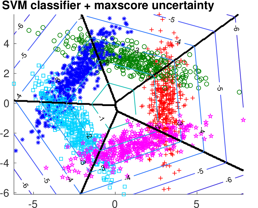
A common heuristic based on using the maximal SVM score \(s(x) = \psi(x)^T w_{h(x)} + b_{h(x)}\).
-
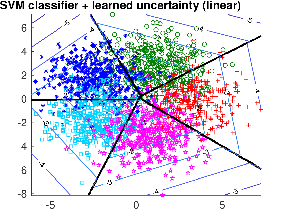
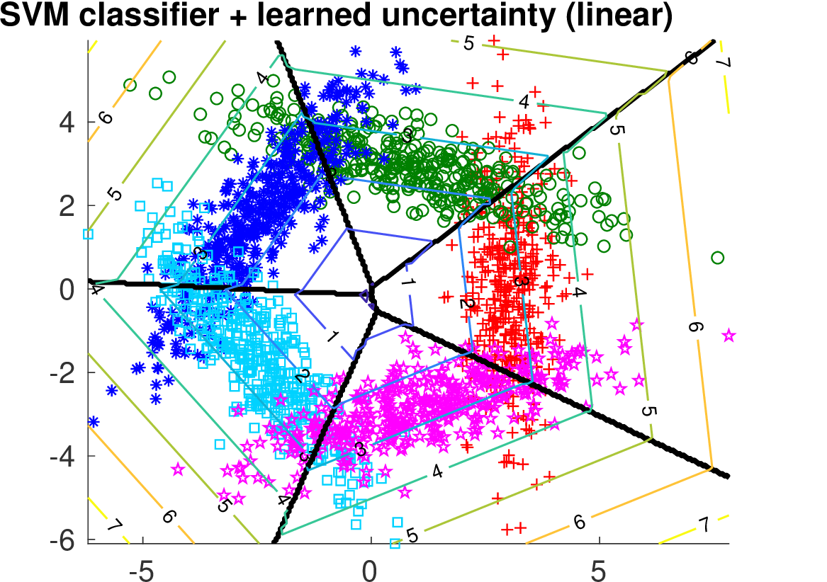
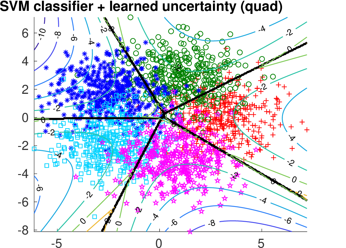
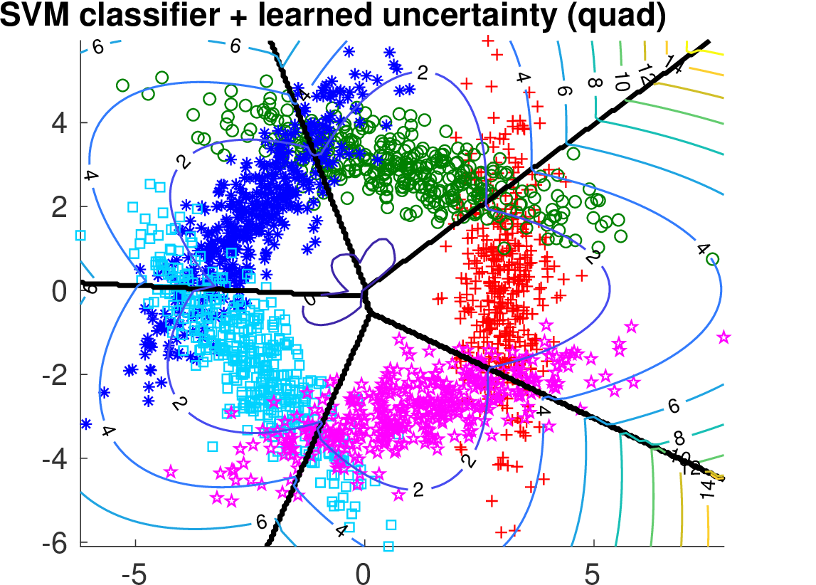
We use a linear uncertainty function \(s(x) = \psi(x)^T u_{h(x)} + v_{h(x)}\) and learn its parameters \((u_{y},v_y), y\in\cal{Y}\), by minimizing the SELE loss. We use linear and quadratic feature maps \(\psi(x)\).
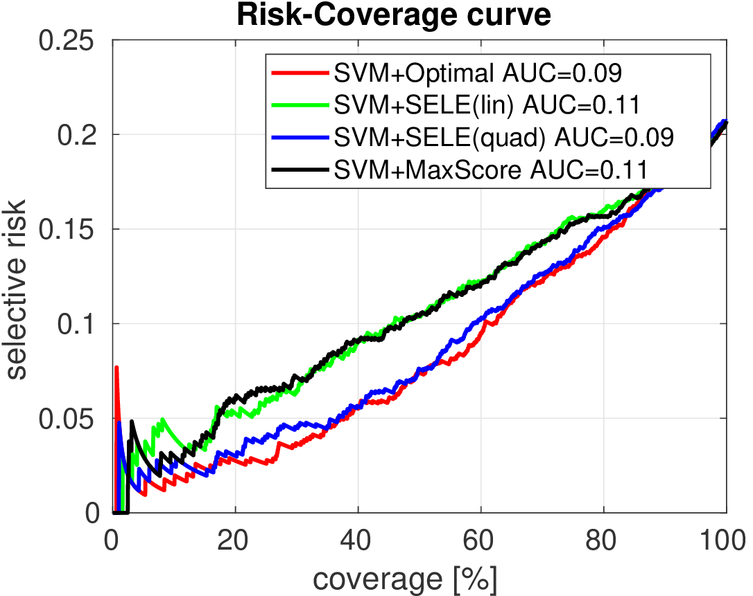
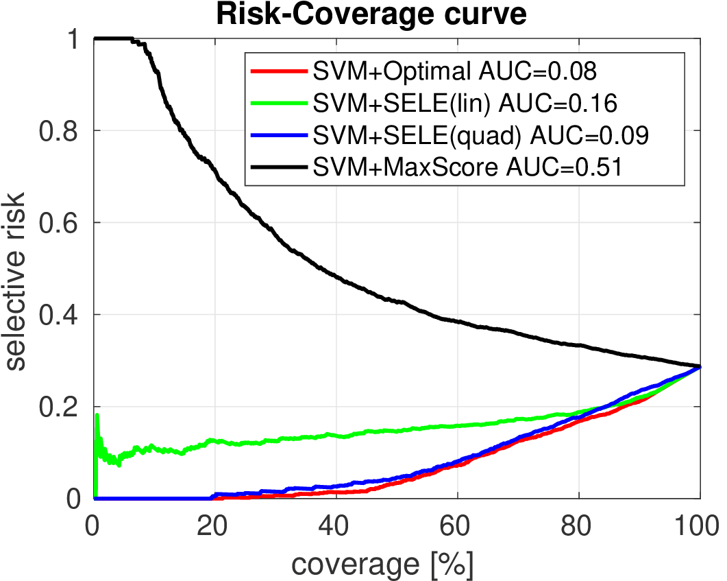
We compare the two methods on two synthetically generated classification problems. Having the data generating distribution allows to construct the optimal selection function. Both classification problems have 5 classes generated from 2D Gaussians whose mean vectors are placed on a circle. In case of Data 1, covariance matrices are spherical. In case of Data 2, the principal Eigen vector of each covariance matrix is tangential to the circle.
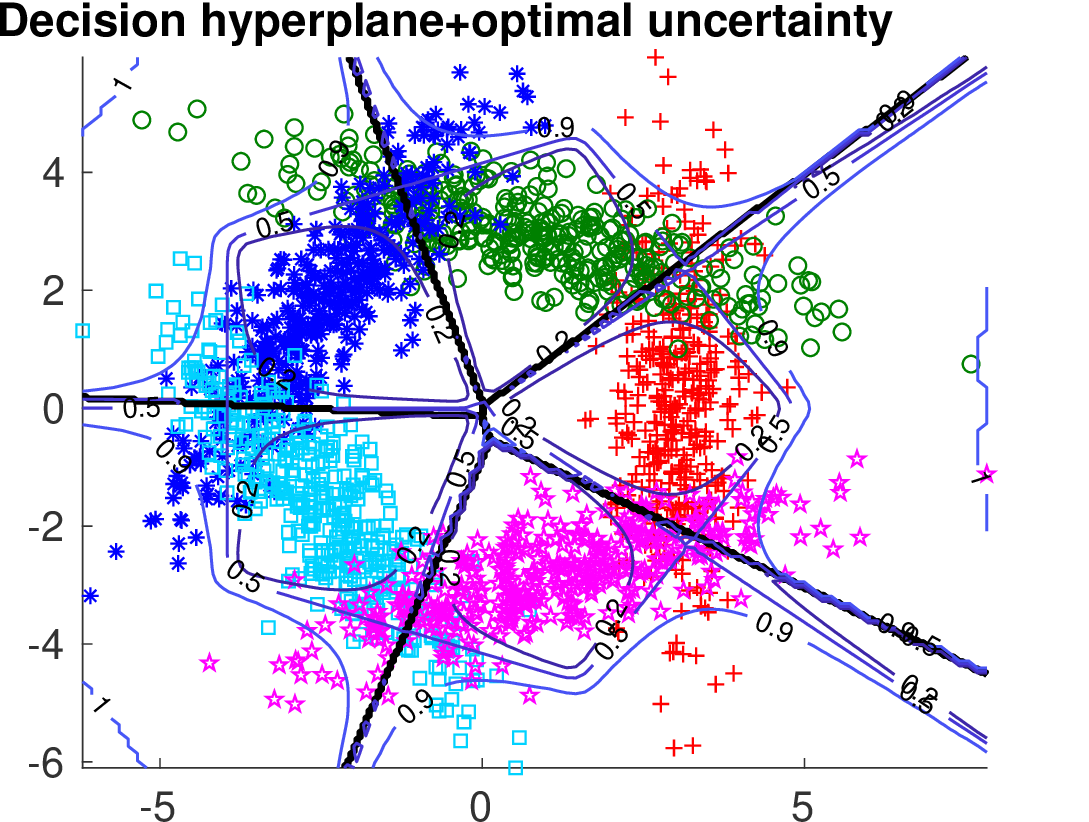
Below we show the Risk-Coverage curves and the area under the RC curve for all compared selective classifiers. We also visualize the SVM classifier (the same for all methods) and the contours of the corresponding uncertainty function.
It is seen that on Data 1 the max-score heuristic is a reasonable approximation while on Data 2 it completely fails unlike the learned linear uncertainty function. In addition, using a more flexible quadratic function we can learn the uncertainty approaching the optimal solution.
For results on real-life data see the paper [Franc & Prusa, 2019].
| Data 1 | Data 2 |
|---|---|
 |
 |
| selection function |
Data 1 | Data 2 |
|---|---|---|
| optimal |  |
 |
| max-score | 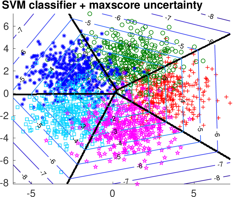 |
 |
| learned linear |
 |
 |
| learned quadratic |
 |
 |
Code
Matlab implementation at GITHUB.